User manual

About this manual

Coverage Pro RF predicts radio coverage over real terrain for land-mobile and amateur systems: repeaters, base stations, links and the subscriber radios that use them. This manual explains every screen and setting, how the predictions are made, and how to use them for common jobs such as checking a new repeater, comparing antennas and running an interference study.

It is written for the radio technician who knows feedlines, duplexers and antenna data sheets but is not a propagation specialist. The How it works chapter goes deeper for those who want the background.

Conventions

• Bold names a button, tab or setting exactly as it appears on screen.
• Signal levels are in dBm (power into 50 Ω) and µV (voltage across 50 Ω). Antenna gains are in dBi.
• Bearings are degrees true unless marked M (magnetic).
• Distances and heights follow the units chosen in Settings → Preferences: feet and miles, or meters and kilometers.
• Infrastructure means the fixed stations you are planning: repeaters, bases and links on towers.
• Subscriber radios are the mobiles, portables and control stations that use them.

Quick start: your first coverage map

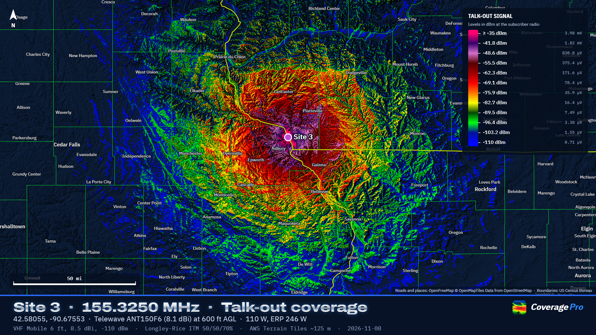
1. Add the repeater. On the Infrastructure tab click Add site, then click the map where the tower is (or type the coordinates into the search box first). Click the Repeater preset.
2. Fill in the station. Set the antenna height above ground, the output frequency, the transmit power and the system losses (feedline, duplexer, connectors). Choose the antenna from the Antenna list.
3. Set up the map. On the Coverage tab, tick the repeater, choose Talk-out, pick the subscriber radio (Mobile is the default) and set the radius.
4. Run it. Click Run coverage. A Normal map of a 30-mile radius takes well under a minute on a typical computer.
5. Read and style it. Right-click anywhere on the map to read the predicted signal there. On the Map tab, adjust colors, smoothing and relief; nothing re-runs.
6. Share it. On the Map tab click Make presentation map sheet for a finished image, or use Export for Google Earth.

Your work saves automatically on this computer. Use Save for a project file you can open elsewhere or send to someone. This manual opens from Help in the top bar or with F1. Save as PDF… at the top of the manual (or Help → Save Manual as PDF… in the menu) saves a printable copy.

The window at a glance

The main window: the panel on the left, the map on the right, the toolbar along the top of the map.

Top bar

Project name, New, Open, Save, Export, Library, Help, the Settings gear and the light/dark switch.

Panel tabs

Infrastructure (your sites), Coverage (set up and run a map), Map (how the result looks), Interference (C/I studies) and Link (point-to-point paths).

Map toolbar

Site and Probe modes, the Tools menu (Measure, Aim antenna, Terrain profile, Range rings) and Hide coverage. The search box on the right finds a place or goes to typed coordinates.

Cursor readout

The bar at the lower left shows the position under the mouse, its grid square, ground elevation, and distance and bearing from the selected site.

Projects

A project holds your sites, coverage and interference settings, model settings and any saved layers. Type a name in the box at the top left. New clears the current project (click it twice to confirm) and starts one from your new-project defaults (see Preferences). Open loads a project file; Save writes one. Older Coverage Pro RF projects open unchanged: their thresholds, colors and antennas keep the values they were saved with. The half-circle button switches between dark and light themes.

Infrastructure tab

The Infrastructure tab: the site list on top, the selected site's editor below.

Each site is one radio at one location with its own transmitter, receiver and antenna. Most are repeaters or bases; you can also add a mobile or portable as a site to test a particular path on the Link tab.

Adding sites

Add site

Turns on Site mode: click the map where the station is. You can also right-click any point and choose Add site here. Drag a marker to move a site.

From library

Opens Library → Infrastructure sites, where Add to project drops in a site you saved earlier, complete with its antenna.

Import CSV

Reads a spreadsheet with a header row. Only latitude and longitude are required (columns named lat/latitude and lon/long/longitude). It also reads name or callsign, height, frequency or output, power, system losses, antenna (model name, matched against the built-in antennas), gain (dBi), mount (top or side), azimuth, downtilt and receiver threshold (µV if positive, dBm if negative), so RepeaterBook exports work directly. A height column labelled (ft) or (m) is read in that unit; otherwise heights use your units setting. Anything left out gets the Repeater defaults.

Sample CSV

Saves an example file with every column Import CSV reads, filled in for a few stations.

Name, color and presets

Type the site's name at the top of the editor; the colored circle beside it sets the marker and map color. The preset buttons (Repeater, Base station, Mobile, Portable, Point-to-point link) fill in typical height, power, losses, threshold and antenna. Change anything afterward.

Station settings

Latitude / Longitude

Decimal degrees, WGS84. Negative longitude is west.

Antenna Height

Height of the antenna's center of radiation above the ground at the site, not above sea level. Ground elevation comes from the terrain data. For a collinear, use the middle of the radiating section.

Frequency

Transmit frequency in MHz. For a repeater, its output. Talk-in maps use the same path loss as talk-out (see Talk-out and talk-in), so the input frequency is not needed.

Transmit power

Power out of the radio or amplifier, in watts, before the feedline.

System Losses

Everything between the transmitter and the antenna: feedline, duplexer, combiner, isolators, jumpers and connectors, in dB. The same loss applies on receive. 2 to 4 dB is common for a duplexed repeater.

Receiver threshold / Same threshold

The weakest signal this site's receiver can use, in dBm or µV; editing either updates the other. Used for talk-in maps and link margins. New sites start at −110 dBm (0.71 µV), the same as subscriber radios; a receiver's 12 dB SINAD sensitivity is lower (0.25 µV is −119 dBm, 0.35 µV is −116.1 dBm), so −110 leaves a working margin.

Choosing the antenna

The Antenna list holds My antennas (ones you saved) and the built-in antennas, grouped by manufacturer with their published gain per band in dBi. Pick one and its figures fill in. To keep the list short it shows only antennas made for the site's frequency; tick Show antennas for all frequencies to see every one (the setting is remembered). The note under the list says where the antenna came from:

• For a built-in antenna, where its figures come from: the manufacturer's pattern file, the manufacturer's catalog, a dealer listing, or not yet checked against a data sheet. Check the data sheet for antennas marked that way or marked as having disagreeing sources. From my antennas: unchanged from your library.
• Changed from … for this site: you edited a figure. Save as a new antenna keeps your version in My antennas under a name you type; Update … in my antennas overwrites your saved entry (only for your own); Undo changes goes back to the library figures.
• Entered for this site only: you chose Enter my own… at the bottom of the list. Pick the Antenna type and type the figures, then Save to my antennas if you will use it again.

Pointing direction, mount and mechanical tilt belong to the installation, so switching antennas keeps them. See Antennas in depth for how each type is modeled.

Antenna figures

Gain

Peak gain in dBi. For a built-in omni the published gain for the site's band fills in; editing it re-fits the pattern and marks the antenna changed. If a data sheet gives dBd, add 2.15.

Vertical beamwidth (optional)

For an omni you entered yourself. Leave blank to estimate it from the gain.

Top of tower / Side of tower

Top assumes a clear mount with an even pattern. Side models an antenna off the side of a tower: stronger in the direction it Faces (degrees true), weaker behind by the Front-to-back figure (6 to 10 dB is typical).

Electrical downtilt

Degrees the main beam is tilted down by the antenna's design (phasing), for omnis.

Downtilt / Mechanical downtilt

Degrees a directional antenna is physically tilted down.

Pointing (azimuth)

Direction a directional antenna points, degrees true. The Aim antenna tool can set it for you.

Front-to-back

How much weaker the antenna is directly behind than in front, in dB.

Horizontal / vertical beamwidth

Half-power (−3 dB) widths of a directional antenna. They are estimated from gain; type over them with the data-sheet figures.

Load pattern file

For the Pattern file type: reads Planet/MSI (.msi, .pln) and .ant pattern files.

The Top view and Side view drawings show the resulting pattern. The line under them shows EIRP (power after losses and antenna gain, relative to isotropic), ERP (relative to a dipole, 2.15 dB lower) and the threshold in µV.

Site buttons

Link from here

Opens the Link tab with this site as the transmitter.

Coverage from here

Ticks only this site and runs a coverage map.

Save to library

Keeps the site (location, height, power, losses, threshold and antenna) in Library → Infrastructure sites so you can add it to other projects. Saving a site whose name is already in the library updates that entry.

Delete site

Removes the site from the project (click twice to confirm). Saved library copies are not affected.

Antennas in depth

Built-in antennas

The built-in list holds about 300 repeater, base and directional antennas from Antenna Specialists, Celwave/Phelps Dodge, Comet, Comprod, Cushcraft, dbSpectra, Decibel Products, Diamond, E/M Wave, Hustler, Kathrein Scala, Laird/Antenex, L-com, Motorola, PCTEL/Maxrad, Sinclair, Telewave, TRAM/Browning and TX RX Systems, plus generic omnis (dipole, ground planes, collinear) and generic yagi, panel and corner reflector types. All gains are in dBi. Directional antennas carry their gain and, where published, horizontal and vertical beamwidth. Exposed-dipole antennas with an offset pattern carry their published offset gain, which is used when the site's mount is set to side. Each omni carries its published gain for every band it is specified for; the band matching the site's frequency is used. If an antenna is not specified for the site's frequency, the editor warns and uses the nearest band's figures. You can hide built-in antennas you never use in the Library.

How omni patterns are built

Manufacturers publish gain and often vertical beamwidth, rarely the full pattern. Coverage Pro RF models each omni as a stack of half-wave dipoles whose number and spacing are fitted to the published gain and beamwidth. That gives realistic main lobes, side lobes and the nulls under high-gain antennas, which matter close to a tall site. The note under the antenna fields shows the model used, for example "4 stacked elements at 0.75 λ, 16° vertical beamwidth". Published amateur-antenna gains are often optimistic. Lowering them by 1 to 2 dB gives a more conservative map; save the result as your own antenna so you use the same figure every time.

Side mounting

An omni mounted off the side of a tower radiates more in the direction it faces and less behind, because the tower reflects and blocks part of the signal. Side mounting models this with a cardioid-like horizontal pattern set by the Front-to-back figure. Exposed-dipole antennas such as the Telewave D-series and DB224 default to side mounting with their published offset gain.

Directional antennas

Yagi, panel and corner reflector types use the gain, beamwidths and front-to-back you enter. Beamwidths left at their estimates follow the gain. Point them with Pointing (azimuth), or use Tools → Aim antenna to get the bearing to a town, hill or other site and apply it.

Pattern files

For measured patterns choose Enter my own…, set the type to Pattern file and click Load pattern file. Planet/MSI files (.msi, .pln) and .ant files in all three common layouts (360 azimuth values, 541 values, or the full 720) are read. Save the result to My antennas to reuse it.

Coverage tab

The Coverage tab sets up and runs a map.

Transmitting sites and direction

Tick one or more sites. When one site is ticked, selecting a different repeater or base on the Infrastructure tab (or clicking its marker) moves the tick to it, so the next map is for the station you're working on. When several sites are ticked, for example a whole system, selecting one to edit leaves the ticks alone. With several sites, each point on the map shows the best one. Unticking a site after a run takes its coverage off the map at once; ticking it again brings it back without recomputing.

Talk-out

Can the subscriber hear the repeater? Levels are at the subscriber radio's receiver.

Talk-in

Can the repeater hear the subscriber? Uses the subscriber's transmit power and the repeater's receiver threshold. Levels are at the repeater receiver.

Both ways

Shows only places where both directions work, colored by the weaker one.

Subscriber radio

Pick the subscriber radio from your Library: Mobile, Portable and Control station come with the program, and you can add your own. To see or change its antenna height, gain, cable loss, receive threshold and transmit power, open Change for this project, or edit it in the Library.

Change for this project lets you adjust those figures for this project only. The note then offers Update … in my library (make the change permanent), Undo changes, or for a radio from someone else's project, Save to my subscriber radios.

Antenna height

Above ground. A mobile roof antenna is about 6 ft (1.8 m); a portable at the hip about 5 ft.

Antenna gain

dBi. A quarter-wave on a roof is about 2 dBi; a portable's antenna at the hip is about −3 dBi or worse.

Cable and connector loss

Between the radio and its antenna.

Receive threshold

The weakest signal the subscriber radio can use. The default is −110 dBm (0.71 µV), a practical working level for FM with some fade margin; change it in the Library to match your standard.

Transmit power (talk-in)

Used for talk-in and both-ways maps.

Vehicle and building penetration losses are not offered: they vary too much from vehicle to vehicle and building to building to predict usefully. Maps show outdoor signal at the subscriber antenna height.

Area and detail

Radius

How far from each site to compute.

Map detail

How many points are computed across the map (grid method): Draft for trying ideas, Normal for most work, High and Ultra for final maps (several times longer).

Advanced

Click Advanced to open these. Most maps never need them.

Method

Grid computes a square grid of points across the map. Radial computes along radials from the site, every Azimuth step degrees, at every Range step along each, then draws the result. Radial shows the most terrain detail (drainages, bluffs, slopes facing the site) and takes longer: run time grows with the square of the radius. Interference maps always use the grid.

Terrain detail

How finely terrain is sampled for the map. Automatic uses about 3,000 × 3,000 points over the area; High uses up to 5,000 × 5,000 and the finest data available.

Azimuth step / Range step

Radial spacing. 0.1° (3,600 radials) with terrain spacing (about 30 m) matches the finest detail the model uses.

Running and updating

Run coverage starts the map; the button becomes Stop while it runs, and the line under it shows progress, then the time taken, the number of points and the terrain source used. Colors, layers and base map → Map tab appears when the map is done. Direction, the subscriber radio's gain, loss, threshold and power, and everything on the Map tab update instantly without recomputing. Changing a site's height, power, antenna or location, or the subscriber antenna height, needs a new run: maps that took under 15 seconds update by themselves, and slower ones show Map out of date with an Update map button.

Map tab

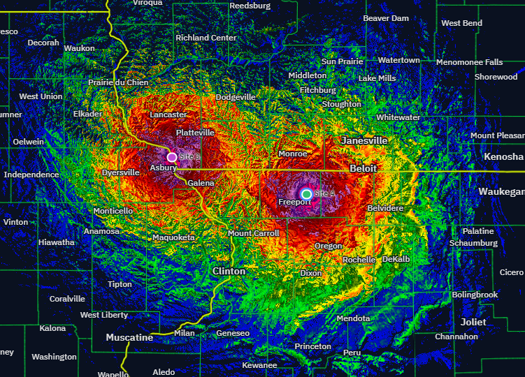
The Map tab: everything here changes the picture instantly.

Saved layers (system coverage) After a coverage run, Keep this map as a layer saves it. Do this for each repeater or group, then choose Saved layers combined: each point shows the strongest signal from any ticked layer, so a linked system can be built up one machine at a time. Tick or untick layers to change what is included; Remove deletes one (click twice). Latest run goes back to the most recent map. Colors, direction and the subscriber radio's gain, loss, threshold and power apply to combined layers without recomputing. The subscriber antenna height is fixed when each map is computed, so make layers with the same height; the panel warns if they differ. Layers are kept on this computer between sessions and saved inside the project file.

Colors and levels

Presentation (navy) / Overlay on map

Presentation turns areas without coverage navy and shows terrain as embossed relief, the style for map sheets. Overlay colors only covered areas so the base map shows through.

Bands / Gradient / Strongest site

Bands: each color covers a range of levels, from its own level down to the next. Gradient: the same colors blended continuously. Strongest site: each site gets its own color, showing which repeater a subscriber hears best.

Color scheme

Coverage Pro RF (the default): 12 colors from −35 dBm down to −110 dBm, about 6.8 dB apart. Also: Classic, signal (red to green), spectrum, thermal, Repeater Blue and a colorblind-safe scheme.

Number of colors

3 to 12, spread evenly between the strongest and weakest levels.

Strongest level / Weakest level

The dBm values of the first and last colors. Nothing is drawn below the weakest level. Weakest = receiver threshold sets it to the threshold in use so every colored area is usable. To make your own levels the default for new projects, use Settings → Preferences.

Editing levels

Type a new dBm value for any row or click its swatch to choose another color; the scheme then shows as Custom. Reset colors to scheme undoes your edits.

Appearance

Smoothing

Off draws every computed point exactly as calculated (sharp squares when zoomed in). Light blends between neighbouring points. Medium, Strong and Max also soften pixel-level noise. Smoothing changes only the picture; probe readings are always the computed values.

Terrain relief / Exaggeration

Relief shades hills and valleys; exaggeration multiplies their height so gentle terrain still shows.

Opacity

How solid the coverage colors are in Overlay style. Presentation style always draws them at full strength, exactly as the legend and map sheets show them.

Outline the coverage edge / Thin lines between colors

A light line around the edge of coverage, and thin lines between bands (Bands view).

Base map and reference layers

The layers button at the top right of the map chooses the background (Navy for presentations, Topographic, Streets, Satellite or OpenTopoMap) and turns these layers on and off for the project: Roads, County and state outlines, Town names and Hillshade.

Roads, outlines and town names

Coverage Pro RF draws these itself, so you choose how they look. Each row has Show, a Color, a Width (text size for town names) and an Opacity from 5 to 100%, so roads and outlines can be faint enough to read the coverage through them:

• Interstates and freeways, US and state highways, Main roads and County and local roads (local roads appear as you zoom in).
• County outlines and State outlines. Dashed county outlines switches the county lines between dashed and solid.
• Town names: cities at every zoom, towns, villages and hamlets as you zoom in; names never overlap.

Wide lines get a thin dark edge so they stand out over the coverage colors. The styling is yours, not the project's: it applies to every project and to map sheets and batch maps. Back to the standard colors resets it.

Roads and town names come from OpenStreetMap through OpenFreeMap (shown as "OpenFreeMap © OpenMapTiles Data from OpenStreetMap" on the map and on sheets) and need an internet connection. County and state outlines come from US Census Bureau boundary files built into Coverage Pro RF, so they work offline.

Map sheet

Make presentation map sheet opens the map sheet window (see Map sheets and exports).

Interference tab

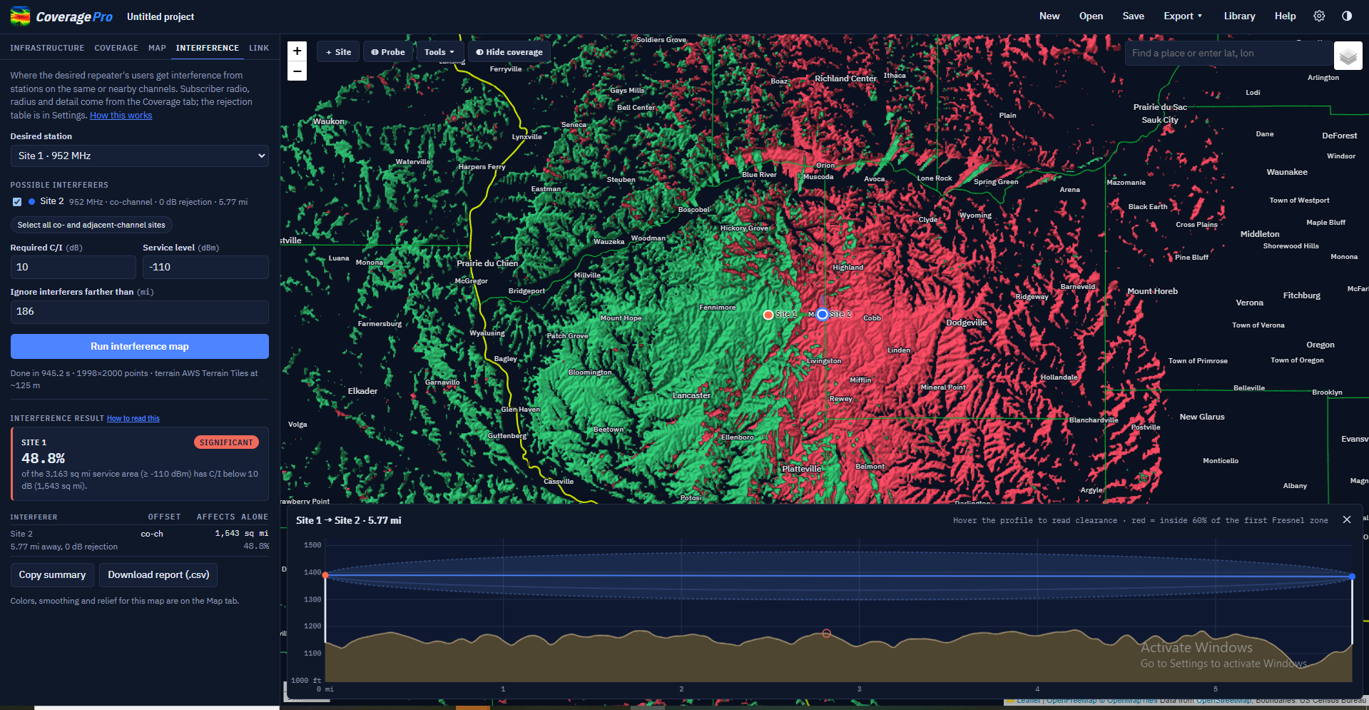
An interference study: setup on top, the result below.

Checks whether other stations on the same or nearby channels degrade a repeater's service. The study uses talk-out signals: the desired repeater's output against the other stations' outputs, as heard by the subscriber radio chosen on the Coverage tab. The radius and map detail also come from the Coverage tab.

Setting up

Desired station

The repeater whose service area is being protected.

Possible interferers

Every other site, with its frequency offset, the rejection that offset gets, and its distance. Sites too far off channel for the rejection table are greyed out, and a site on the same channel within 300 m is flagged as a probable duplicate. Select all co- and adjacent-channel sites ticks every station within the table.

Required C/I

How much stronger the desired signal must be than the combined interference, in dB. 10 dB is a common analog FM figure; use your coordination standard.

Service level

The desired signal level that counts as service. Weaker places are outside the service area and aren't judged. It defaults to the subscriber threshold; set it to your protected-contour level if you use one.

Ignore interferers farther than

Limits how far away interferers are counted.

Run interference map

Computes the study. The rejection table is in Settings → Interference rejection.

Reading the result

The result shows the share of the service area with C/I below the requirement, and for each interferer the area it would affect by itself. On the map, green is protected service and red is service with interference; on the Map tab, By interferer colors each interfered spot by the station causing most of it. Copy summary copies a one-paragraph result for an email; Download report (.csv) saves the table.

Required C/I, service level, the rejection table and the subscriber radio's figures update the result instantly; changing sites or the radius needs a new run.

Link tab

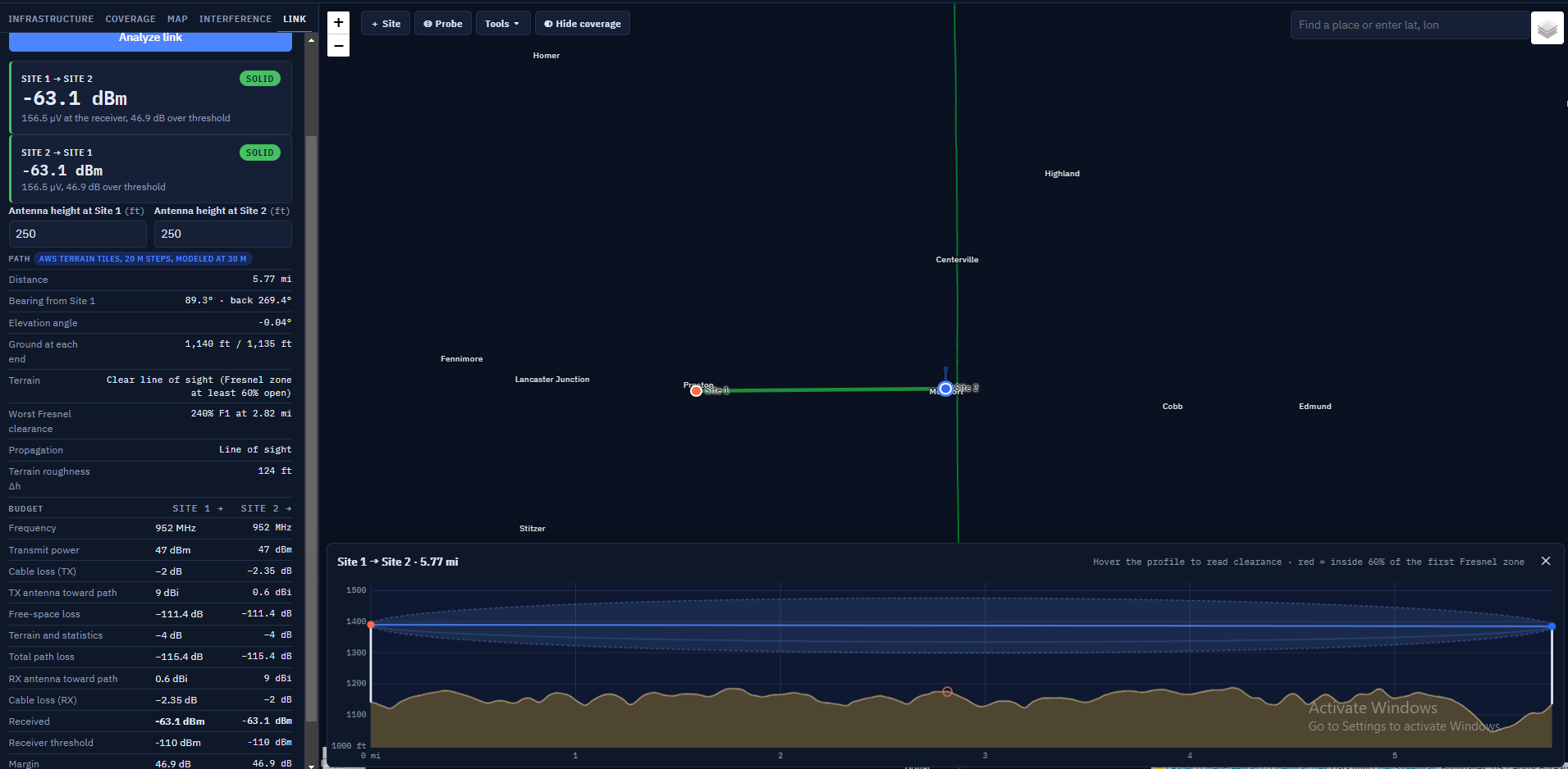
A link analysis with its terrain profile.

Analyzes the path between two sites, in both directions, using the same model, terrain spacing and antenna patterns as coverage maps.

Choosing the path

Pick From (transmits) and To (receives); ⇅ swaps them. After you probe a point on the map, Map point appears in the To list: a subscriber radio at that spot with the Coverage tab's figures. Click Analyze link.

Reading the result

Verdict

Solid: at least 10 dB above the receiving station's threshold. Marginal: 0 to 10 dB above. No link: below the threshold. Both directions are shown.

Path

Distance, bearing both ways, elevation angle, ground at each end, line of sight, worst Fresnel clearance and propagation mode (line of sight, diffraction or troposcatter).

Budget

Every gain and loss from transmitter to receiver. "Terrain and statistics" is the loss beyond free space from obstructions, ground effects and the chosen reliability.

Antenna heights

The antenna height at each end, right in the result. Type a new height and the whole result and profile update at once, without reloading terrain. The height is the site's own height, so it also applies to its coverage maps. The same instant update happens when you change a site's power, losses, threshold or antenna on the Infrastructure tab.

Copy summary / Show profile

Copy a one-paragraph result, or reopen the profile drawer.

The profile

The profile draws the terrain with earth curvature for the k-factor in Settings. The straight blue line is the direct path and the shaded band is the first Fresnel zone; red marks terrain inside 60% of it. At least 60% of the first Fresnel zone should be clear to avoid extra loss. Hover the profile to read ground height and clearance; a marker follows on the map. A warning appears when ground close to either antenna rises above it, since the model averages terrain over 30 m steps and may under-count a close obstruction.

Map toolbar and tools

The Aim antenna tool with a directional antenna's beam drawn on the map.

Site, Probe, Hide coverage and search

Site

Click the map to add a site there.

Probe

Click the map to read the predicted signal: talk-out and talk-in levels with their margins, the ground elevation, and for interference maps the C/I and strongest interferer. Right-clicking does the same at any time. The popup offers Add site here and Link from …, which runs a link from the site whose coverage reaches that point.

Hide coverage

Hides the coverage to show the map underneath without losing the result. The H key does the same.

Search

Type a place name, or coordinates as "lat, lon", and press Enter.

The Tools menu

Click Tools and choose a tool; its name then shows on the button. Each tool opens a small panel. Click the tool again, click ✕ on its panel, or press Esc to close it. While a tool is on, clicking a site marker uses that site's exact position.

Measure

Click points to measure distance and bearing leg by leg, with the total and the straight-line distance from start to end. Double-click or right-click to finish. Each leg shows its bearing and back bearing, true and magnetic. Copy copies the legs as text; Terrain profile (one leg only) profiles it; Clear starts over.

Aim antenna

Choose the site in Antenna on, then click where its antenna should point: a town, a hill or another site. The panel shows the azimuth (true and magnetic), distance, the look angle up or down to a subscriber radio there (or the far antenna, for a site), the antenna's −3 dB beamwidth and its edges, and how far off the current setting is. Drag the yellow target to fine-tune. Point … at …° writes the azimuth into the site, and the coverage map updates. A top-mounted omni has no pointing direction, so the button is not offered for one.

Terrain profile

Click the start, then the end. Sites use their own antenna height; points use the subscriber radio's. Change the heights and frequency in the panel. It shows distance, bearing, ground at each end, the worst first- Fresnel clearance and a verdict, and draws the profile in the drawer. Full link analysis runs the Link tab between the two ends when at least one is a site.

Range rings

Click a site or any point to draw distance rings around it. Type the distances in Ring distances, separated by commas. Rings around a site follow it when it moves, stay after the tool closes and are saved with the project. Remove takes one center away; Clear all rings removes them all.

Cursor readout

Shows the position under the mouse (decimal degrees), its 6-character Maidenhead grid square, the ground elevation from the terrain tiles, and the distance and bearing from the selected site.

Magnetic bearings

Magnetic bearings use the World Magnetic Model (WMM2025, valid to the end of 2029) at the start of each line, for today's date. Magnetic = true − declination; east declination is positive. Towers, vehicles and buildings can throw a compass off by more than that, so take compass readings away from steel.

Library

The Library: antennas, infrastructure sites and subscriber radios that are yours in every project.

Click Library in the top bar. The Library belongs to you, not to a project: it is there in every project you open. A project that uses a library entry carries its own full copy, so it opens the same on a computer that doesn't have your library.

Antennas

My antennas lists the ones you saved, with Edit and Delete. + New antenna adds one from a data sheet: name, type (omni, yagi, panel/sector, corner reflector), gain in dBi, and for directional antennas the horizontal and vertical beamwidths and front-to-back (left blank, they are estimated from the gain); for omnis, the optional vertical beamwidth and electrical downtilt. Pattern-file antennas are saved from a site's editor and can be renamed here.

The built-in antennas follow, grouped by manufacturer. Hide removes one from the Antenna list on your sites (projects already using it are not affected); Show … hidden built-in antennas lets you bring them back.

Infrastructure sites

Sites saved with Save to library from the site editor. Add to project adds one to the current project with its antenna; Delete removes it from the library (click twice).

Subscriber radios

Mobile, Portable and Control station to begin with, each with antenna height, antenna gain, cable and connector loss, receive threshold (dBm or µV) and transmit power. + New subscriber radio, Edit, Delete and Make default (the radio new projects start with).

Sharing a library

Export… saves your whole library as a file (coverage-pro-library.json). Import… adds the entries from such a file to yours; entries already present are updated. Use it to share antennas and sites with another coordinator or to move to a new computer.

Settings

Settings opens from the gear in the top bar.

Click the gear at the top right. Terrain data, Propagation model and Interference rejection are saved with the project. Preferences are yours and apply to every project.

Terrain data: elevation

In the United States, terrain comes from USGS 3DEP, lidar-derived bare earth down to 1 m where flown. Coverage Pro RF downloads only the area and resolution each job needs. Elsewhere, or when USGS can't be reached, it uses AWS Terrain Tiles (about 30 m worldwide); choose AWS Terrain Tiles only to always use them, which is faster. The status line shows which source is connected. Add .hgt files loads your own SRTM tiles, which take priority where they cover; Remove unloads them.

Terrain data: land cover

Bare-earth data leaves out trees and buildings. Use USGS NLCD land cover adds them from the National Land Cover Database (30 m classes) for coverage and interference maps in the US; link analysis stays bare earth.

Trees and buildings block the path

Adds a typical clutter height for each class to the terrain along every path (forests 15 m, woody wetlands 12 m, developed land 6 to 15 m; the heights are editable). A tree line or town between the repeater and the subscriber then shadows the signal like a hill. The first and last 60 m of each path stay bare, so the antennas themselves aren't buried.

Extra loss when the subscriber is among trees or buildings

When the subscriber radio is inside a forest or town, the signal also has to get down through the clutter around it. This uses the ITU-R P.2108 terminal clutter model, counting only the loss beyond what the propagation model already includes for open ground: typically 2 to 7 dB at VHF and UHF.

Propagation model: terrain and climate

Ground type

Electrical properties of the ground (permittivity and conductivity). Average ground suits most farmland and prairie.

Radio climate

Continental temperate covers most of the US interior.

Surface refractivity

How much the atmosphere bends radio waves, in N-units. 301 is standard; 250 to 400 is the valid range.

Polarization

Vertical for FM repeaters and most land-mobile; horizontal for SSB and weak-signal work.

Earth factor k

Used only for drawing link and terrain profiles. 4/3 (1.333) is standard; a lower k shows a more pessimistic earth bulge.

Propagation model: statistics

How certain the prediction should be. 50% is the median; higher percentages give weaker, more conservative predictions.

Variability mode

How the percentages combine. Mobile (the default) treats time and location variability together, which fits a subscriber moving through the area. Broadcast treats them separately, for a fixed receiver. Accidental and Single message are for interference studies.

% of time

Fading over hours and seasons.

% of locations

Spot-to-spot variation within a small area.

% of situations

Confidence in the model itself for paths like this one.

Interference rejection

How much a receiver rejects a signal at each frequency offset: co-channel 0 dB, 7.5 kHz about 3 dB, 15 kHz about 35 dB, and so on. Stations beyond the last row are ignored in interference studies. Edit the rows to match your coordination standard; Add row adds one and Reset to typical values restores the defaults.

Preferences

Units

Feet and miles, or meters and kilometers. Signal values stay in dBm and µV.

S-units

Off by default. FM radios' S-meters aren't calibrated to a standard, so the same signal can read S1 on one radio and S6 on the IARU scale. Show S-units adds them next to dBm and µV, on the IARU standard (S9 = −93 dBm above 30 MHz, 6 dB per S-unit), the HF scale (S9 = −73 dBm), or your own S9 level and dB per S-unit.

Prepared by

Text added to the third caption line of map sheets, such as your organization's name.

New-project defaults

The map colors' strongest and weakest levels and the subscriber radio every new project starts with. The program's defaults are −35 to −110 dBm (12 colors) and a Mobile at −110 dBm. Use this project's map levels copies the current project's levels; Back to the program's defaults resets them. Projects you already saved keep their own values.

Map sheets and exports

Presentation map sheet

A finished PNG with the coverage, roads and labels, site markers, legend, scale bar, north arrow and a three-line caption that fills in from your settings and can be edited before saving. Size offers 1920 × 1080 for screens and slides, letter or 11 × 17 at 300 dpi for printing, and a square format. Extent is the whole coverage area or the current map view. Tick or untick roads, county and state outlines, town names, distance rings and the legend. Roads, outlines and town names use your colors from the Map tab, and the sheet credits the map data sources. The licensee's name appears on every sheet.

Export menu

Presentation map sheet (.png)

Opens the map sheet window.

Coverage for Google Earth (.kmz)

The coverage as a ground overlay plus site placemarks.

Coverage overlay image (.png)

The transparent coverage image by itself.

Interference report (.csv)

The table from the last interference map.

Sites list (.csv)

All sites and their settings, for a spreadsheet.

Sites and last link (.kml)

Site placemarks and the most recently analyzed path.

Batch maps

Export → Batch maps for many repeaters… (or File → Batch Maps, Ctrl+B) makes finished maps for many repeaters at once, for a website or handouts. Choose the repeaters from this project (Select all / Select none) or a CSV file such as a RepeaterBook export (Choose file…), pick a folder (Choose folder…), choose which maps (talk-out, talk-in, two-way, and an interference study wherever other stations share or neighbor the channel), the radius, detail and sheet size, and whether to draw roads, towns and distance rings. Click Start batch. For every repeater you get map sheets with thumbnails, transparent overlays and Google Earth files, plus a summary with coverage area by color level. Each run also writes a gallery page (index.html) with a searchable list and map, and a combined interference spreadsheet. The maps use this project's subscriber radio, color levels, land cover, interference rules, model settings and S-unit setting. Every repeater and base in the project counts as a possible interferer, even if it isn't ticked. The run happens in the background. Repeaters that haven't changed since the last run into the same folder are skipped unless you tick Redo. Open gallery and Open folder appear when it finishes.

How it works

The propagation model

Coverage Pro RF uses the Longley-Rice Irregular Terrain Model (ITM 1.4, point-to-point mode), the US standard for VHF and UHF terrain propagation, implemented from the NTIA reference code and checked against it. It is valid from 20 MHz to 20 GHz and 1 to 2,000 km. For each path, ITM looks at the terrain profile between the antennas, finds the radio horizons, and blends line-of-sight, diffraction and troposcatter losses with the ground's effect. The statistics settings then set how conservative the answer is.

Terrain spacing used by the model

ITM was designed for terrain sampled tens of meters apart. Given lidar-fine profiles, a road bank or ditch beside a low antenna becomes its "horizon" and the model adds diffraction loss that isn't real. So every map, probe and link is modeled with terrain averaged over 30 m steps (the spacing of SRTM 1 arc-second data). Metre-scale bumps are averaged out; valleys, ridges and drainages stay in. Results are the same whatever the terrain detail, radius or screen.

Talk-out and talk-in

Radio paths are reciprocal: the path loss from the repeater to a point equals the loss from that point back. Coverage Pro RF computes the path loss once and applies each direction's transmitter, receiver and antenna figures.

Talk-out level at a point = repeater power − repeater system losses + repeater antenna gain toward the point − path loss + subscriber antenna gain − subscriber cable loss.

Talk-in level at the repeater = subscriber power − subscriber cable loss + subscriber antenna gain − path loss + repeater antenna gain toward the point − repeater system losses.

Talk-out is compared with the subscriber's receive threshold; talk-in with the repeater's. A 50 W mobile against a 50 W repeater with the same thresholds gives nearly the same map both ways; a 5 W portable is 10 dB weaker on talk-in, which is why many systems are talk-in limited. The repeater is assumed to receive through the same antenna and feedline it transmits on, as with a duplexer.

Antenna patterns in the calculation

For each point the program works out the azimuth and elevation angle from the antenna to the point (with earth curvature) and reads the pattern there. That is how downtilt, side mounting, directional antennas and the nulls under high-gain omnis show on the map.

Interference math

For each point in the desired station's service area, each interferer's signal is reduced by the rejection for its frequency offset, the interferers are added as powers, and the desired signal is compared with the total. Where the ratio is below the required C/I, the point counts as interfered.

Signal units

dBm

Power relative to 1 milliwatt. −80 dBm is a strong mobile signal; −110 dBm is a practical working level for an FM subscriber radio; −116 dBm is near the limit of a typical FM receiver.

µV

The same level as voltage across 50 Ω, as on receiver spec sheets. 1 µV = −107 dBm; 0.71 µV = −110 dBm; 0.35 µV = −116.1 dBm.

Margin (dB over threshold)

How much stronger than the weakest usable signal. 10 dB or more leaves room for fading and obstructions.

dBi / dBd

Antenna gain relative to an isotropic source or a half-wave dipole. dBi = dBd + 2.15.

EIRP / ERP

Transmit power after losses and antenna gain, relative to an isotropic antenna (EIRP) or a dipole (ERP, 2.15 dB lower).

Limits of any prediction

A prediction is a statistical estimate from terrain data, not a measurement. It does not know about individual buildings, vehicles, local noise, intermodulation, desense or a damaged feedline. Use margins, compare with drive tests where you can, and keep the statistics settings consistent between studies you compare.

Workflows

Checking a new repeater application

1. Add the proposed site from the application: location, antenna height, ERP (set power, losses and antenna to match), output frequency.
2. Run talk-out coverage with the Mobile subscriber radio at the radius your standard uses, and note the service contour (the weakest color that counts as service).
3. Import or add the existing stations on and near the channel, then run an interference study on the Interference tab with your required C/I and service level. Repeat with the new station as an interferer to the existing ones.
4. Use Copy summary and Download report for the file, and make a map sheet for the applicant.

Comparing antenna options

1. Run coverage with the first antenna and click Keep this map as a layer on the Map tab.
2. Choose the second antenna in the site editor; the map updates or shows Update map.
3. Toggle between Latest run and the saved layer, or right-click the same points to compare levels.

System coverage for a linked network

1. Run each repeater (or each group) and keep each as a layer.
2. Choose Saved layers combined and tick the machines in the system. Strongest site shows which repeater serves each area best.
3. Make a map sheet of the combined system.

Aiming a link or sector antenna

1. Set the site's antenna to a directional type.
2. Tools → Aim antenna, choose the site and click the far end (a site marker snaps to it).
3. Click Point … at …°. Use the magnetic bearing with a compass on site, away from the tower steel.
4. Check the path with Tools → Terrain profile or the Link tab.

Troubleshooting and questions

The map is smaller than I expected

Check the subscriber radio's threshold and gain, the weakest color level (nothing is drawn below it), the statistics percentages (higher is more conservative) and whether land cover is on. A portable at the hip covers far less than a mobile.

Talk-in is much smaller than talk-out

That is usually real: the subscriber has much less power than the repeater. A better receive antenna, lower duplexer loss, a receiver preamp or voting receivers improve it.

"Map out of date"

You changed something the map depends on. Click Update map; small maps update by themselves.

Terrain says AWS instead of USGS

USGS couldn't be reached or the area is outside the US. Maps still work at about 30 m. Check the internet connection, or choose AWS only in Settings for speed.

An antenna I used is missing from the list

It may be hidden: in Library → Antennas, click Show … hidden built-in antennas.

A project from someone else shows "from another library"

The site uses an antenna saved in their library. The figures are in the project, so results are the same; click Save to my antennas to keep it.

Probe readings differ slightly from the colors

Smoothing changes only the picture; probe readings are the computed values at that point.

The program is slow

Use Draft detail while setting up, Grid instead of Radial, and a smaller radius. Very large Ultra maps and many saved layers use a lot of memory.

What's new in this version

1.3.2

• About 625 more built-in antennas (Comprod, Kathrein Scala, PCTEL/Maxrad, Telewave, Decibel and others), including directional ones. Each says where its figures come from, and the list shows only antennas made for the site's frequency unless you tick Show antennas for all frequencies.
• A site you add by clicking the map, or from the library, becomes the only site ticked for the next coverage run.
• Zooming no longer pauses while county and state outlines draw: each map tile draws only the outline pieces that cross it.
• Map sheets: the title is set in a wide silver face, the Coverage Pro RF icon sits beside the brand mark, and the coverage is drawn at the same resolution as on screen so sheets look like the map.

1.3.1

• Automatic sharpening removed: it kept the processor busy after every zoom.
• When one site is being mapped, selecting a different repeater or base moves the coverage map to it.
• New repeaters and bases start with a −110 dBm receiver threshold, like subscriber radios (saved sites keep theirs).
• Opacity for each kind of road, the outlines and town names (Map tab).
• Link analysis updates at once when you change an antenna height (now right in the link result) or any radio setting of either end.
• The summary line under the subscriber radio list is gone; its figures are under Change for this project.

1.3.0

• New default colors: 12 colors from −35 to −110 dBm.
• Presentation style shows the colors at full strength on screen, so the map matches the legend and map sheets.
• The base map and layer choices are back on the map (the layers button at the top right).
• Roads, county outlines, state outlines and town names are drawn by Coverage Pro RF in your own colors and widths, on screen, on map sheets and on batch maps.

1.2.0

• New layout: Infrastructure, Coverage, Map, Interference and Link tabs; expert coverage settings under Advanced; Settings in their own window; map tools under one Tools menu.
• The Library: your antennas, infrastructure sites and subscriber radios, available in every project, with import and export. The built-in antennas are included; hide the ones you don't use.
• Subscriber radios (Mobile, Portable, Control station) replace the old user presets.
• New default: subscriber receive threshold −110 dBm and map colors down to −110 dBm, both changeable in Preferences.
• Vehicle and building loss options removed.
• This manual, also available as a PDF from the Help window.

1.1.9

• Map tools: Measure, Aim antenna, Terrain profile, Range rings, cursor readout, magnetic bearings (WMM2025).

Updates

Coverage Pro RF checks for a new version shortly after it starts and every few hours while it runs. A new version downloads in the background; when it is ready you can Restart now or choose Later, and it installs the next time you close the program. Help → Check for Updates… checks right away. Your license, library, settings and saved layers are kept. Save your project before restarting if you have unsaved changes.

License and copyright

Coverage Pro RF is Copyright © 2026 Coverage Pro RF. All rights reserved. Coverage Pro RF and its logo are trademarks of Coverage Pro RF.

Your copy is licensed to the person named in Help → About Coverage Pro RF, and that name appears on every map sheet. The license is for your use only: don't share your key or copy the software for others. Maps you make are yours to use and publish. The full terms are in the license agreement under Help → About. Coverage Pro RF uses open-source components and public data, each under its own license. They are listed under Third-party notices in Help → About.